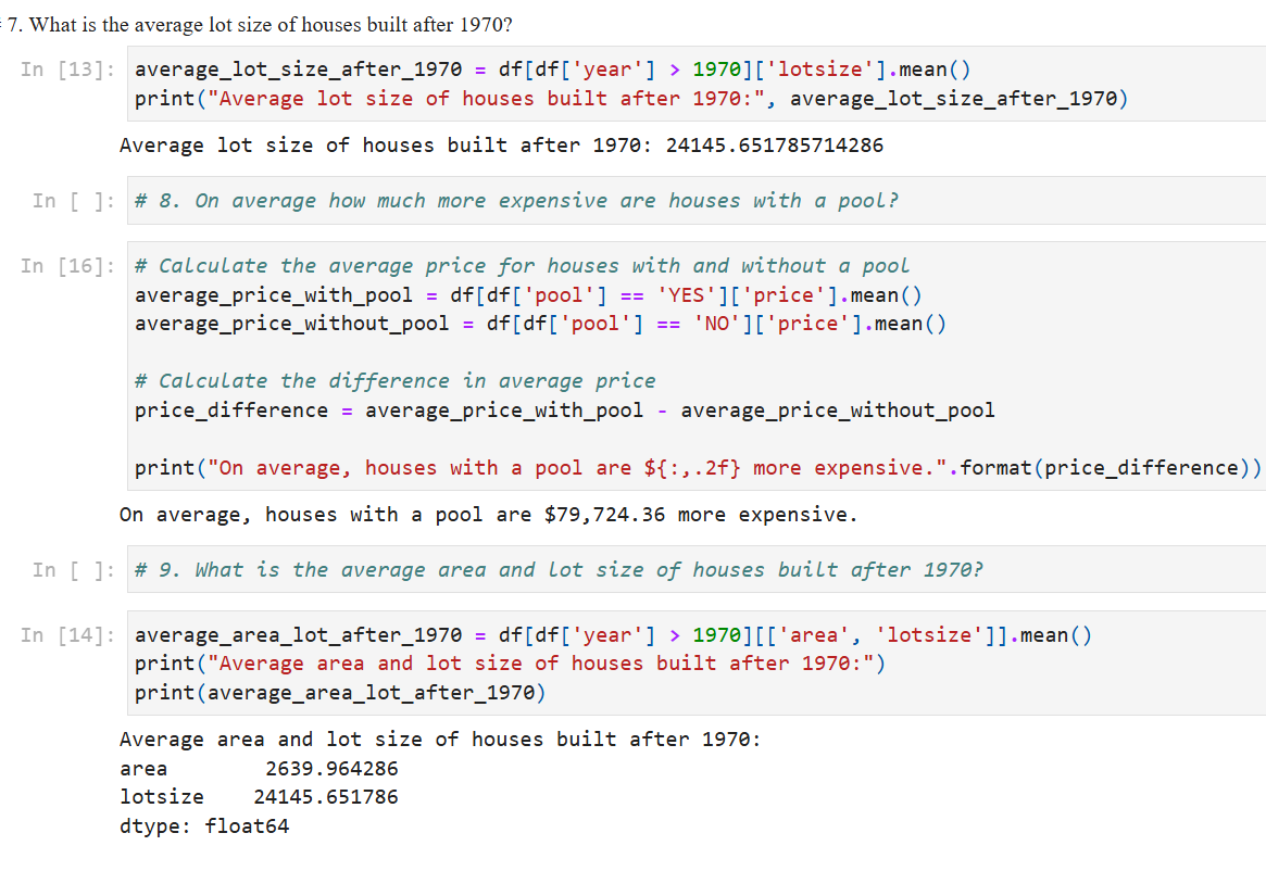
The objective of this python script is to estimate house prices from a large US city. The real estate data is initially in the form of a .csv file with each row containing the attributes of the house. We can identify statistics from the data, such as the average lot size of houses built after 1970, or the average difference in price between houses with a pool versus houses without a pool.
Machine Learning Models
Counterfeit Identification
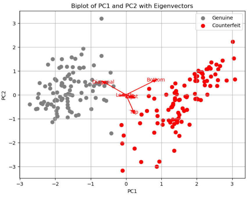
This graph is from an assignment where I was given a data set containing measurements from genuine and counterfeit Swiss franc bank notes. In order to find which variables are useful to identify counterfeits, I first found the principal components from the dataframe and create a scatterplot of the PC1 and PC2 values. Then I find the eigenvalues and explained variance. I then display the eigenvectors on the scatterplot to create a biplot. From the data given in this assignment, the diagonal measurement is the most useful to identify counterfeit bank notes.
Data Visualization
Prediction Models
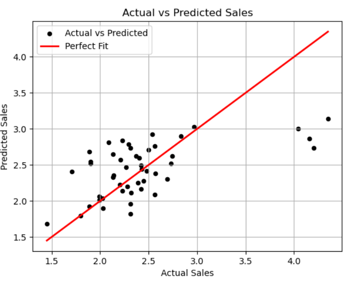
In this assignment, I was given medical and insurance data including the patient’s age, sex, body mass index (bmi), children, smoker (yes or no), region and the total medical expenses charged to the plan during the year. I built a regression model with the predictors in order to predict annual medical expenses for patients. I created new binary variables for obese patients and smokers, and reported how much more expensive an obese patient is compared to a non-obese patient, and how much more expensive a smoker is compared to a non-smoker. This scatterplot shows the actual expenses and the predicted expenses.
Web scraping and data analysis in Python
This is an extracurricular project that I developed outside of school because I wanted to learn basic web scraping, and at the same time practice some data science skills I learned at UTSA.
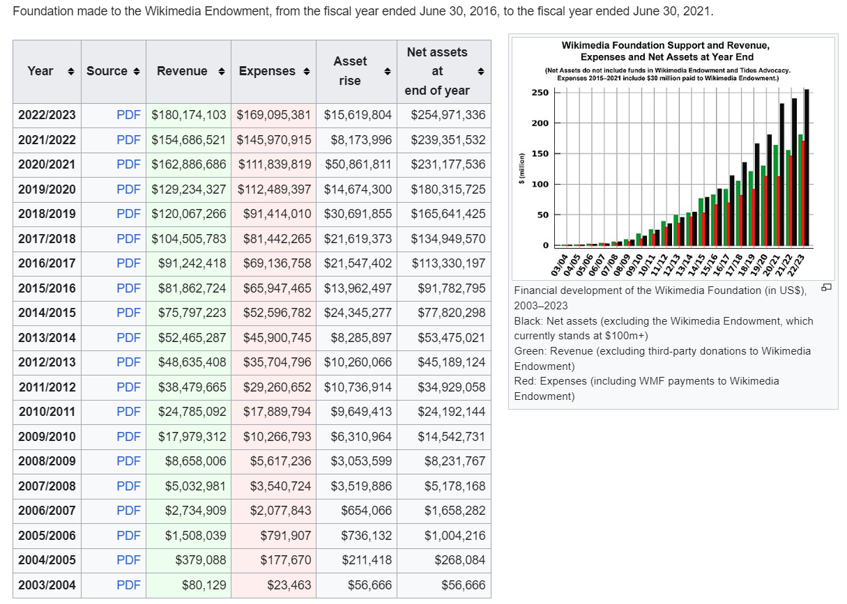
I first import the data science library Pandas, then use .read_html() to collect the data from the HTML table on the Wikipedia web page, save it as a pandas data frame, and make a copy in order to leave the original data unchanged.
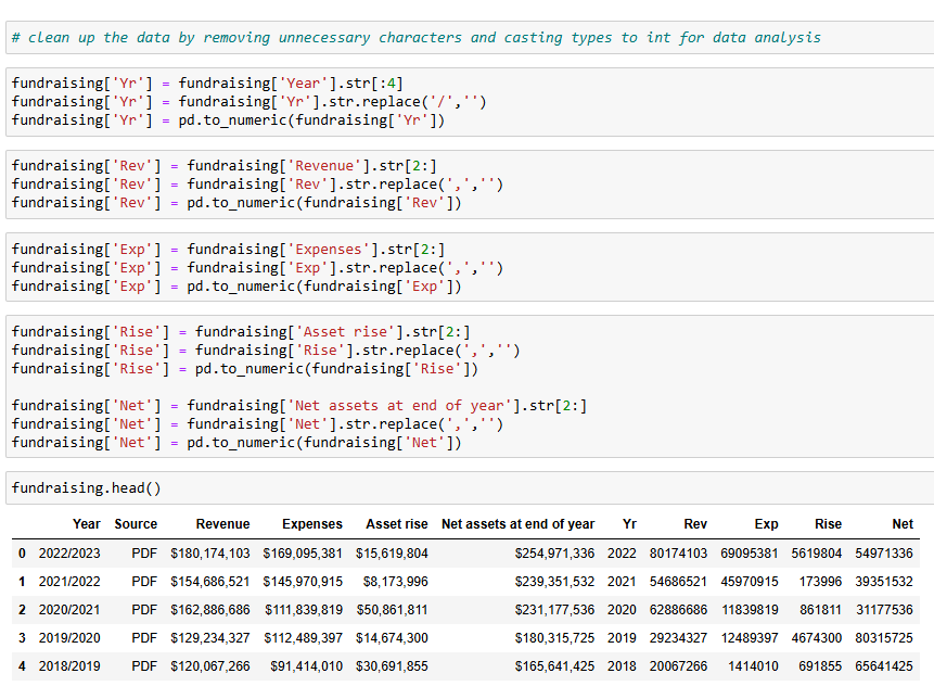
I then clean and prepare the data for analysis by removing unnecessary characters using str.replace() and convert strings into integer data types using .to_numeric().
With the unnecessary characters removed and types converted, I can perform mathematical operations on the data.
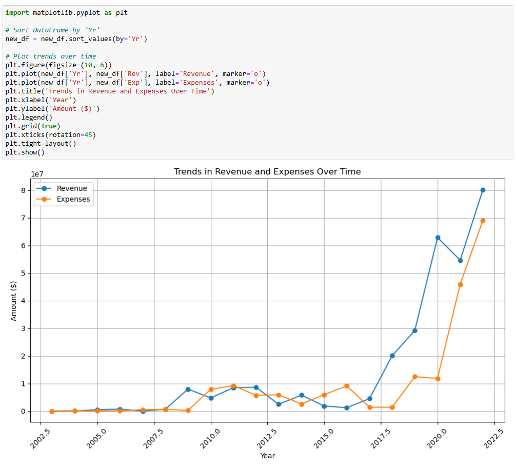
I then use matplotlib.pyplot to display a plot of revenue and expense trends over time.
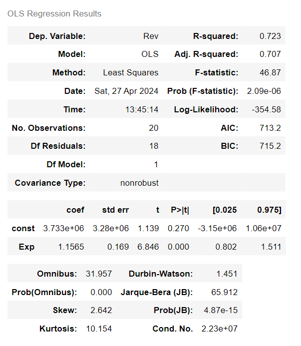
I also use numpy, statsmodels, and sklearn to split the variables up using revenue as the response and expenses as the predictor, and perform an ordinary least squares regression analysis to predict revenue based on expenses, and then calculate the year-over-year growth rate of revenue and expenses.
The results of the OLS analysis tell us that for every additional dollar spent on expenses, the model predicts that revenue will increase by approximately $1.1565.
An R-squared of 0.723 indicates that approximately 72.3% of the variance in revenue can be explained by expenses in this model. The coefficient for ‘Exp’ is 1.1565, meaning that for every one unit increase in expenses, revenue is predicted to increase by approximately 1.1565 units. The p-value for ‘Exp’ is very low, indicating that expenses is a significant predictor of revenue.
I also performed feature engineering by calculating the year-over-year growth rate of Revenue and Expenses. Value is Not a Number for the first row because there is no previous value to compute the percentage change.
Finally, I export the data frame as a csv file for later analysis. You can see the entire python script on my GitHub profile:
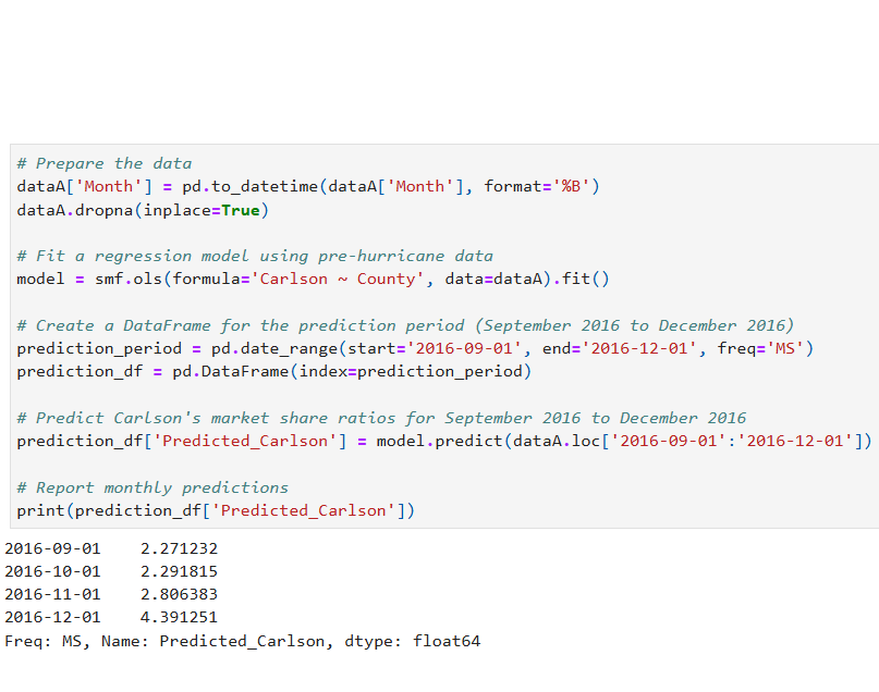
This is a python script that I wrote as part of a data mining and machine learning course I took at UTSA. This scenario occurred after a hurricane struck the east coast. More than $8 billion in federal disaster relief and insurance money came into the county, resulting in increased sales at department stores and numerous other businesses. The Carlson Department Store was closed for four months due to heavy damage, and was involved in a dispute with its insurance company about the amount of lost sales during the time the store was closed. Two key issues needed to be resolved: The amount of sales Carlson would have made if the hurricane had not struck, and whether Carlson is entitled to additional compensation for the loss of increased sales after the storm.
I first import some data science libraries: pandas, numpy, matplotlib, sklearn, scipy, statsmodels. The original data is a .csv file, so I read it into a dataframe, and make a copy of it in order to leave the original data unchanged. I then find the ratios of Carlson monthly sales to the county-wide department stores monthly sales. This is Carlson’s historic market share. Then I use pre-hurricane data (2016-Aug 2020) to fit a regression model to predict Carlson’s market share ratios from Sep 2020 to Dec 2020.
I then multiply the county monthly sales (Sep 2020 to Dec 2020) times the predicted Carlson’s market share ratios and report them along with their sum. Carlson could potentially demand this amount from the insurance company.
The insurance company might argue that the predicted market share ratios or the multiplication of these ratios with county monthly sales data do not accurately reflect the actual losses incurred.
A second approach is to find county departmental stores excess sales due to the hurricane impact. This can be accomplished by creating ratios (of county sales predictions to actual county sales) after the hurricane hit. These are called excess ratios since they show how much sales existed when compared with regular monthly sales if no hurricane hit.
First, I fit a regression model to predict monthly county-wide sales, then find ratios of actual vs. predicted monthly county-wide sales, these are the excess ratios. Next, I use pre-hurricane data to fit a regression model to predict the loss of regular sales (had there been no hurricane) for Carlson Store.
To display how well the model fits the data, I display a line plot of actual and estimated Carlson’s sales had there been no hurricane. I then multiply the excess ratios by Carlson Store predicted sales from Sep 2020 to Dec 2020. Carlson can demand this amount from the insurance company.
Cancer Classification Models
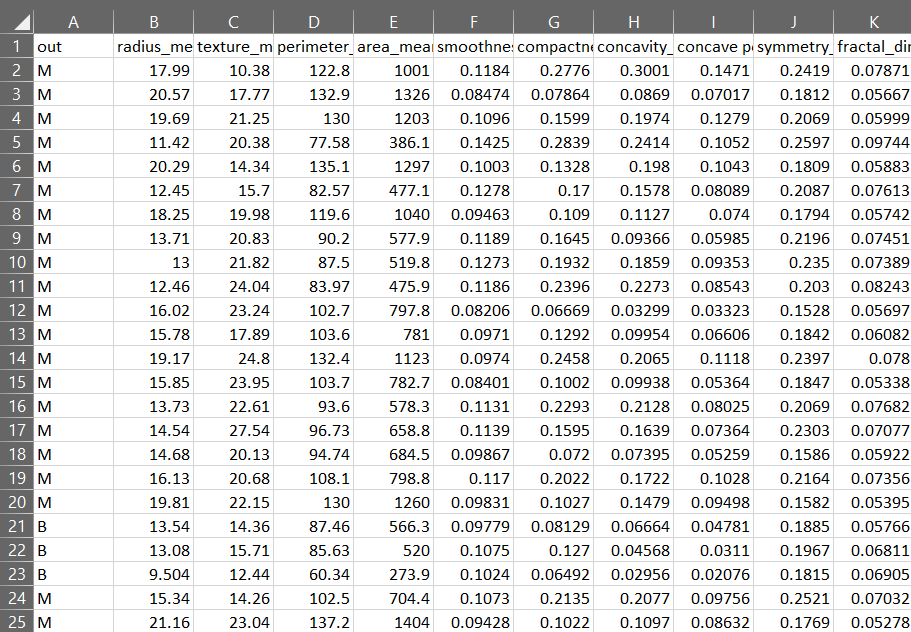
The objective of this assignment is to build classification models with a high accuracy rate for patients with cancer. The raw data is a .csv file containing lab results from patients with a tumor, each labeled as benign or malignant.
The dataset includes 30 lab measurements (predictors) associated with breast cancer tumors. We want to predict the variable 'out'. This is a binary classification problem since the variable to predict has two categories (M,B).
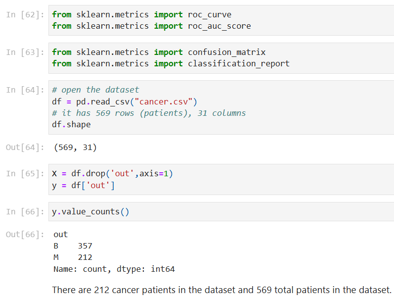
I begin by importing some python data science libraries: numpy, pandas, matplotlib, and sklearn, then I read the .csv file into a pandas dataframe. Using .shape, we can see that the dataset has 569 rows (patients) and 31 columns (lab measurements). I then split the data into train and test (stratified) sets, and use the train set to build a KNN model.
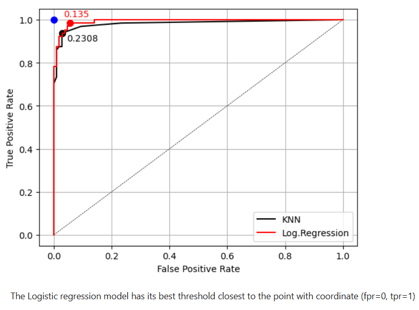
There are many false positive rates and true positive rates, so we use them to create a line plot. We want the highest possible true positive rate, while also keeping the false positive rate low. We can identify the point that is as close as possible to the top left corner of the graph (the best threshold).
I then use the train set to build a logistic regression model and plot the ROC curve and find the best threshold. We can then compare the two models by finding the area under the curve (AUC) of the KNN model and the logistic regression model. Using AUC for comparison, the Logistic Regression model is best, and has the best threshold.
Counterfeit Principal Component Analysis
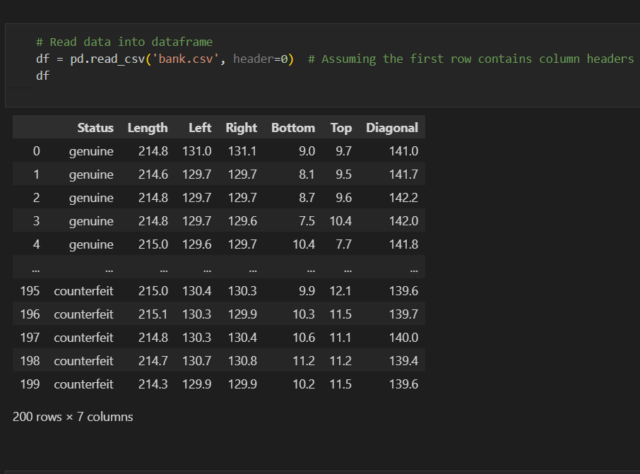
For this assignment, we want to know which variables are useful to identify if a bank note is counterfeit. Finding principal components and a biplot may help. The file bank.csv contains six measurements made on 100 genuine and 100 counterfeit old-Swiss 1000- franc bank notes. For each bank note it has the following variables:
Status (categorical): genuine or counterfeit
Length: The length of the bill (mm)
Left: The width of left edge (mm)
Right: The width of right edge (mm)
Bottom: The bottom margin width (mm)
Top: The top margin width (mm)
Diagonal: The bill’s diagonal length (mm)
I scale the data by subtracting the mean and dividing by the standard deviation for all the columns, then find all six principal components from df, display a scatterplot of PC1 and PC2 values, and find the eigenvalues and show the rotation matrix of all six principal components.
'Bottom' is more useful for identifying counterfeit bank notes, despite its lower correlation, because its direction aligns with counterfeit points in the biplot. The direction of the eigenvector for 'Diagonal' in the biplot suggests that it contributes more to the detection of genuine rather than counterfeit bank notes.
Real Estate Statistics
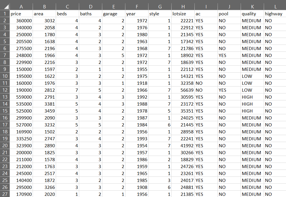
The objective of this python script is to estimate house prices from a large US city. The real estate data is initially in the form of a .csv file with each row containing the attributes of the house.
First, I import the data science libraries numpy and pandas and read the .csv file into a dataframe. I can now count, filter, and sort the data easily to find information such as:
The most expensive house with at least three bedrooms, or
The least expensive house of a particular style.
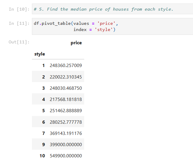
Pivot tables can be used to find information such as: the median price of houses from each style.
We can identify statistics from the data, such as the average lot size of houses built after 1970, or the average difference in price between houses with a pool versus houses without a pool.
Relational Database Design: Restaurant Schema in SQL
This is a database that I designed and implemented as a project in my Database Systems class while earning my Computer Science degree. The design includes an entity-relationship diagram, a schema written in SQL, and several example queries. I explain the use of bridge-entities to solve M:N relationships, normalization, cardinality, ordinality, and ideas for optimization.
 GitHub
 Chaz's Linkedin